

Bayesian Performance Rating: The Best Player Metric in CBB
New updates and a full model technical explainer

With a new season approaching, it’s finally time to dedicate a whole article to the flagship metric at EvanMiya.com, the Bayesian Performance Rating. When I first launched the website in 2020, BPR was the new metric that most provided something unique to the CBB advanced analytics landscape, and I still believe this to be the case today. The player evaluation metric has undergone many iterations as I’ve collected feedback over the years and seen it used in action. BPR has always been useful in its own right, but a lot of other features at EvanMiya.com also depend on it being accurate. Game predictions, lineup metrics, team ratings, injury adjustments, and other tools all use BPR as a key part of their internal formulation.
This offseason, I made some significant upgrades to the Bayesian Performance model that addressed some lingering biases and led to sharper model accuracy. Rather than just mentioning these changes quickly, I wanted to provide users with a complete technical examination of the model so that I can properly convince readers that Bayesian Performance Rating is the best all-in-one player metric publicly available in college basketball.
If you want to skip the explanation altogether, jump to the tables at the end or go view the full datasets on the Player Ratings page at EvanMiya.com.
The Goal of BPR
In a nutshell, Bayesian Performance Rating reflects the offensive and defensive value that a player brings to his team when he is on the court, on a per-possession basis. This rating incorporates aspects such as individual efficiency statistics, on-court impact on team performance down to the play-by-play level, previous career performance, high school recruiting profiles, adjustments for opponent players and teammates, and more. All of this results in one offensive and defensive number, which can be added together to get a player’s overall Bayesian Performance Rating.
Here’s the technical interpretation of BPR:
Bayesian Performance Rating represents how many points per 100 possessions better a player’s team is expected to be than its opponent if that player were on the court with nine other average Division I players. For example, if a player has a BPR of +5.0, this means that if he were playing with average D1 teammates, against average D1 players, his team would be expected to outscore the opposition by 5 points in a 100 possession game.
Typically, the best player in the country each year finishes with a BPR above +10.0, a top 50 player in the country would have a BPR of about +7.0, an average high-major starter would have a BPR of about +4.0, and an average D1 player would have a rating of precisely 0.0.
Part of what makes BPR unique is that it is a predictive stat: BPR doesn’t just summarize how good a player has been in a given season, it actually predicts how productive that player will be going forward. This makes BPR way more useful during a season because you don’t have to wait till February for it to become accurate. Players even have BPR predictions in the preseason, which will start to go up or down as the model updates with current season performance data.
Ultimately, the goal of Bayesian Performance Rating is to get player values that lead to the best future predictions of player and team performance. Every part of the BPR formula has been optimized to achieve the best out-of-sample predictions, employing various cross-validation methods. When a player has a BPR of +6.0, we genuinely believe that he will add about 6 points of value per 100 possessions to his team compared to an average player, based on our extensive testing. There are other commonly referenced player efficiency formulas, such as PER1 or Offensive Rating2, which are human attempts to weigh each part of a player’s box score to measure their overall contribution towards winning. While convenient, these model weights are not determined by rigorous statistical testing and are therefore less reliable for future predictions of player performance.
Here is the formula used for predicting the expected number of points scored in a single offensive possession:
In this equation, i is the intercept representing the average points per 100 possessions in CBB, approximately 104, with a home team advantage adjustment if the game is not played on a neutral court. Each B term represents the coefficient, or BPR rating, for an individual player on offense or defense. If you add up the Offensive BPRs of the five players on offense, and you subtract the Defensive BPRs of the players’ defense, you get the expected points for that possession.
Many model features make BPR particularly effective, which we will unpack in greater detail in a moment:
The model accounts for individual player statistics and advanced box score metrics.
The model measures impact on team performance through analyzing play-by-play outcomes.
The model adjusts for the strength of all other players on the floor for every possession played.
The model is trained on years of Division 1 college data to specifically measure what’s important in the college game.
BPR is a predictive stat, estimating how valuable a player will be going forward.
The model comes with preseason projections for each player, using player historical information to make it more accurate. BPR adjusts up or down as the season progresses, making it useful the entire year.
BPR is bayesian in nature, which allows for preseason priors and measurements of uncertainty around each player’s value estimate.
Model Comprehensive Breakdown
I’m going to explain how each component of Bayesian Performance Rating works. To accommodate readers with varying levels of interest, I will break each part into several sections:
🧭 High-level Overview
🔎 Technical Details
💡 Why It Matters
For those who just want to understand the basics, I’d recommend skipping the 🔎 Technical Details sections.
Model Structure
🧭 High-level Overview
The Bayesian Performance Rating model consists of several individual models that are carefully pieced together. These include my own versions of a regularized adjusted-plus-minus model, a box plus-minus model, and a preseason projection model, all wrapped within a bayesian predictive framework. All three of these model classes are commonly used within basketball for player evaluation, but each has its own shortcomings when deployed in isolation. BPR uses all three model types together to form a superior final version.
🔎 Technical Details
While I will expand on each model type in future sections, I want to briefly describe the individual models and mention their big-picture strengths and weaknesses.
Regularized Adjusted Plus-Minus models3 are a great way to measure a player’s overall on-court impact on offense and defense. It’s basically plus-minus, but adjusting for many of the contextual variables that are lost in basic plus-minus. These models provide valuable information about the value a player brings while on the court, without being biased towards certain player archetypes, like volume scorers or stat-stuffers. A player’s rating considers the scoring outcome of every possession played, adjusting for the strength of both teammates and opposition players faced on each possession.
Without other statistical input, the RAPM model outputs face a variety of issues. Players on very good or very bad teams are often clustered together, since the model can struggle to differentiate between them. Individual games can have a significant impact on the final player coefficients in ways that, without more context added, lead to misleading results. Sometimes players can get “lucky” and end up with a good rating, just because they happened to be on the court during one good team performance and not on the floor during a bad one. A pretty large sample size is needed to get sensible results from the model, so season-level RAPM coefficients aren’t useful till a good portion of the way through the year.
Box Plus-Minus models are an attempt to use box score statistics to create a much more stable version of RAPM. Essentially, a linear regression is performed to determine which box score statistics are most predictive of a good RAPM coefficient. Once these weights are determined, a player’s BPM can be calculated purely using advanced box score stats. BPM models are popular because they are much easier to interpret and understand, and their results are more predictable since they typically align closely with a player’s statistical output.
While BPM models are very convenient, they still leave a lot of valuable player information on the table that’s not captured in the box score. Some players don’t stuff the stat sheet but excel in many other intangible areas, leading to winning outcomes for their team regularly. Other players can score in spades and post ridiculous box scores, but may not actually be “winning” players. Like RAPM, Box Plus-Minus is also not stable with small sample sizes. Typically, BPM leaderboards need to be filtered to show players with a specific possession count to be more trusted. Because of this, BPM is also not very useful early in the season. One other important note: almost all public BPM values come from a formula trained on years of NBA data. While copying this formula and using it for college players is helpful, specific player skills are more valued in the college game, so using an NBA-trained formula leaves a little to be desired (more on that later).
Preseason projection models are not just specific to players, as they are used all across the sports analytics space. Readers will likely be very familiar with college basketball team projections in the preseason, like at EvanMiya.com, KenPom.com, and BartTorvik.com. Similar to how these team projections are formed, a player’s rating in one of these aforementioned player value models can also be predicted using previous season historical data for each player. Naturally, a preseason projection for a player is helpful at the beginning of a season. Still, it should not be viewed as the most accurate representation of a player’s value once we get deeper into the year.
💡 Why It Matters
Bayesian Performance Rating combines three different model types to give the most accurate assessment possible of player value in college basketball. While each of these individual models has significant shortcomings on its own, using their strengths together leads to much better predictions of future player performance, as I have determined from my years of rigorous statistical modeling and testing.
The following several sections will explain how each of these model components works together in greater detail.
Step 1: Multi-Year RAPM Model
🧭 High-level Overview
At its core, Bayesian Performance Rating is a Regularized Adjusted Plus-Minus model. Every Division 1 player is represented by an offensive and defensive coefficient, which measures how much more valuable they are than an average player, per 100 possessions. A coefficient above zero means a player is better than average, and a coefficient below zero means he is worse than average. The model takes an entire season’s worth of play-by-play data across all Division 1 games and adjusts each player’s offensive and defensive ratings until the set of all ratings best explains all the play-level results that have occurred.
🔎 Technical Details
As mentioned in a previous section, the regression equation used in the RAPM model takes the following form:
In a typical linear regression, the possession-by-possession data would be fed into a linear regression engine that spits out the coefficients that make the most sense. However, using a linear regression without “shrinkage” leads to nonsensical coefficients, especially for players who play very few minutes. The standard technique used is to apply some sort of regression to the mean. The simplest way is to use ridge or lasso shrinkage methods to make it difficult for players with low possession counts to be rated way above or below the league mean.
From the inception of Bayesian Performance Rating, I have chosen to use bayesian methods instead, hence the name. Using a bayesian linear regression offers two main advantages. The first is that we can be way more specific about player-level prior distributions. Instead of fixing every player’s prior mean to zero, or some other pre-determined constant, we can choose whatever prior mean and standard deviation we want for each player. As I will explain in Steps 3 and 4, it’s highly beneficial to make the RAPM model more informed by giving each player a starting value that’s a best guess of their coefficient, both in terms of specifying the mean and the amount of uncertainty we have in each player’s prior mean.
When building BPR from scratch, the first step is to create several multi-year RAPM model datasets, each using four years of consecutive data. For example, I used all play-by-play data from the 2021-22 season through the 2024-25 season, treating it as one big season and making a convenient (and wrong) assumption that a player’s value is constant across all seasons played in that multi-year sample. For these models, all players are given the same prior mean and prior variance. While none of these coefficients are actually used for anything public, they do help determine the best amount of prior variance to give to a typical player, which I determined through cross-validation methods. Tuning this parameter through optimization leads to the lowest out-of-sample possession prediction error. Additionally, the multiple years of data led to more stable and trustworthy player coefficients compared to if I had just used single seasons to build the RAPM dataset (which I had done previously).
💡 Why It Matters
Using an advanced plus-minus model on its own only goes some of the way toward building an accurate player metric that predicts future performance. There are some other commonly cited RAPM models used for college basketball, but without a lot more context, I would not feel comfortable trusting these model outputs to guide my own assessments of players. Bayesian Performance Rating is structured like an adjusted plus-minus model, but the model is fed way more information about each player through the form of prior distributions, helping the model make much more intelligent final conclusions.
Step 2: College Box Plus-Minus Model
🧭 High-level Overview
Using the multi-year RAPM datasets from Step 1, I have formed my own college-specific version of a Box Plus-Minus model, called Box BPR. BPM models for player evaluation are powerful because of their intuitive interpretability. A player’s final value is calculated by adding up different statistical box score outputs, each multiplied by some weight that determines how valuable each skill is towards winning. Each rating represents the value that a player adds per 100 possessions to his team. Categories like three-point shooting, assists, and blocks are emphasized, while adverse outcomes like turnovers and missed free throws are penalized. Each player gets an Offensive and Defensive Box BPR based on how valuable their statistical output is, according to the model. These values are used in conjunction with the RAPM model to form more accurate player ratings in Step 3.
🔎 Technical Details
A box plus-minus formula is created by determining how much weight each statistical category should get such that it best predicts overall player performance, team performance, and ultimately, winning. The way this is typically done is by taking offensive and defensive player impact values, calculated through some model that is not biased by box scores whatsoever, and then using the season-level player box statistics to predict those player impact coefficients. The most well-known Box Plus-Minus formula, derived by Daniel Myers4, is trained on several multi-year NBA RAPM datasets. Instead of copying this formula and assuming it is accurate at the college level, I created my own version, called Box BPR, trained on my own multi-year RAPM data from the previous step. All box-stat predictor variables are given to the model on a per-possession basis, such as assists, turnovers, offensive and defensive rebounds, twos, threes, free throws, etc. For example, a player’s rebounding ability would be represented as rebounds per 100 possessions.
Some important executive decisions have to be made about what kinds of predictor variables to give to the model. For example, the average opponent rating faced by each player is used to properly account for competition level. One primary choice I made was to include some measurements of playing time and usage in the model to reward players who play a larger percentage of their team’s minutes and carry bigger offensive loads. If the Box BPR model were only being used in isolation, I might consider using just the per-possession stats without any considerations for playing time or usage. However, since the Box BPR coefficients are used to form each player’s prior mean in the larger RAPM model, giving credit for playing load does make the final BPR model outputs more realistic. Additionally, I do not shift every team’s Box BPR values up or down to add up to the total team efficiency ratings, as is commonly practiced. Doing this skews the final BPR output in undesirable ways.
💡 Why It Matters
While other public Box Plus-Minus models are helpful, the version at EvanMiya.com, Box BPR, is more accurate in college basketball because it is trained on Division 1 data to determine what skillsets are the most valuable at this level. Additionally, since the final BPR model combines the Box BPR values with an adjusted plus-minus model, the box score statistics are properly weighted without relying on them to tell the whole picture about player performance (more on those weights in the next section).
Step 3: Forming a Prior-Informed RAPM Model
🧭 High-level Overview
This is the step where BPR really starts to take shape. Using a bayesian linear regression model allows us to create player-specific prior means, which essentially behave like starting points for the RAPM model. In this case, I use each player’s season-level Box BPR values as a starting point for their offensive and defensive coefficient. For example, suppose a player has an Offensive Box BPR of +3.5 points per 100 possessions. In that case, the model will start by setting the final player's offensive value at +3.5 and then adjust that value up or down based on how that player actually impacted the team's offensive efficiency while on the court. This really helps the model immediately identify the good and bad players, rather than naively giving everyone equal footing to start.
🔎 Technical Details
In our prior-informed RAPM model, we need to get each player’s prior distribution, which will be represented by a normal distribution with a prior mean and prior standard deviation. The prior mean for each coefficient is simply each player’s respective Box BPR rating on offense or defense for the season. The trickier part is figuring out the proper prior standard deviation for each player. I’m not going to reveal all the secret ingredients here, but essentially, the prior standard deviation is determined based on how much of the variation in the RAPM model coefficients can be explained by each player’s Box BPR values. For offense, the Box BPR explains about 50% of the variation in the RAPM coefficients, and for defense, it is about 30%. We can directly use these R-squared values to figure out the exact magnitude of the player prior standard deviations used in the bayesian model.
To make this even more accurate, I actually tested a whole grid of possible global offensive and defensive prior standard deviations to see which ones led to the best out-of-sample possession outcome predictions. I did this partly to see if giving even more weight to the Box BPR priors makes the model more accurate. Turns out, more reliance on these box score priors was useful! Through cross-validation, the best performing offensive prior standard deviation was one equivalent to an R-squared of 66%, and the best defensive prior standard deviation was one equivalent to an R-squared of 59%. What does that mean? When you look at the final BPR ratings, more than half of the weight is given to the box score statistics for most players, with the remaining weight dedicated to the adjusted plus-minus model, which quantifies impact beyond the box score.
Once these prior distributions are determined, the full prior-informed RAPM player ratings can be calculated, leading to full season-level BPR values that incorporate box score stats and adjusted plus-minus modeling.
💡 Why It Matters
Bayesian Performance Rating combines two extremely useful types of data: box score statistics and advanced on-court team impact metrics. Using these in tandem leads to a much more accurate representation of player value, especially when it comes to predicting future impact. The amount of strength given to each of these components is determined scientifically using statistical methods that figure out the proper weighting.
Step 4: Making Preseason Priors
🧭 High-level Overview
The final modeling step is to create preseason projections for each player so that Bayesian Performance Rating is useful from the very beginning of the season. These projections, similar to how team preseason projections are calculated, take a bunch of variables specific to each player to predict that individual’s value for the upcoming season. Variables used include player BPR and Box BPR in previous seasons, high school recruiting profiles, expected developmental growth by class, transfer status, and more. Once these projections are formed, they are also included in the overall BPR model as the season progresses, serving as starting points for each player before any games are played. As a new season unfolds, the BPR values will begin to go up or down based on whether players are performing better or worse than their initial preseason projection. By the end of the year, these preseason projections still carry some weight toward the final BPR ratings, but are far outweighed by the current season box score and team impact metrics used in the model.
🔎 Technical Details
Similar to Box BPR, the goal of the preseason projections is to have a preseason prior distribution for each player. Accurately estimating the prior means is crucial. These starting values have a big effect on BPR outputs early in the season, and they are meant to be useful right away to coaches and fans analyzing player value. There is another equally important step: estimating preseason uncertainty for each player’s prior. Having a unique measurement for preseason uncertainty (prior variance) for each player makes sense. Some players who have been in college for a while are known commodities. They aren’t likely to be a lot better or worse than we expect. Other players are massive wild cards. Highly touted freshmen are erratic, players stepping into bigger roles can be hit or miss, and those who previously missed an entire season may be hard to quantify. Using bayesian modeling techniques for these projections is incredibly valuable because it allows us to obtain a probability distribution for each player that represents all the reasonable outcomes we can expect for how their season will unfold.
I won’t go into much greater detail on how these projection models are built, but I will mention the main factors that contribute to each player’s prior:
Stats and metrics from previous college seasons are used, including BPR, Box BPR, playing time, position, offensive role, and player class. This also accounts for the competition level faced in previous years.
High school recruiting ratings are used, especially for freshmen and younger players, to determine each player's unrealized potential. For example, if two freshmen had similar first-year performances, a 5-star recruit out of high school will have a better sophomore year preseason projection than a 3-star recruit will. Freshmen (and international recruits) projections are constructed by looking at how previous players with similar recruiting profiles have fared in their first year at the D1 level.
Transfer status is also taken into account, which is new to the model this year. I now have two different preseason models, one for returning players and one for transfers. I have found that some metrics are more accurate in predicting player performance for returning players than they are for incoming transfers. For example, advanced On-Off splits are pretty useful for predicting how a player returning to his same team will fare in the following year, but are less helpful for players who change teams and contexts. In general, the transfer model leans more heavily on the box score statistics and less on the other on-court impact metrics.
Once these preseason priors are calculated, I use a bayesian hierarchical model structure to combine the preseason prior with the Box BPR, forming a new, final prior that informs the RAPM model. As the season progresses, the preseason projection portion of the prior will become less influential on the final model outputs. Notably, though, I don’t ever completely erase the preseason data from the model. Since the entire goal of Bayesian Performance Rating is to have ratings that predict future player performance, keeping the preseason priors in, at least to some degree, does really help make better estimates of player value during postseason play. As a general rule of thumb, the preseason priors will carry about 15% of the overall model weight by the end of the season, but this varies greatly player-by-player.
💡 Why It Matters
Having these preseason BPR projections adds significant utility to the model. Not only can we obtain solid estimates of player value before the season even starts, but having these priors influence the model during the season also helps stabilize the model. BPR doesn’t overreact to early performances in the season but uses all available data on each player, including past performances and high school recruiting information, to form the best possible evaluations of players in the present.
Final Numbers
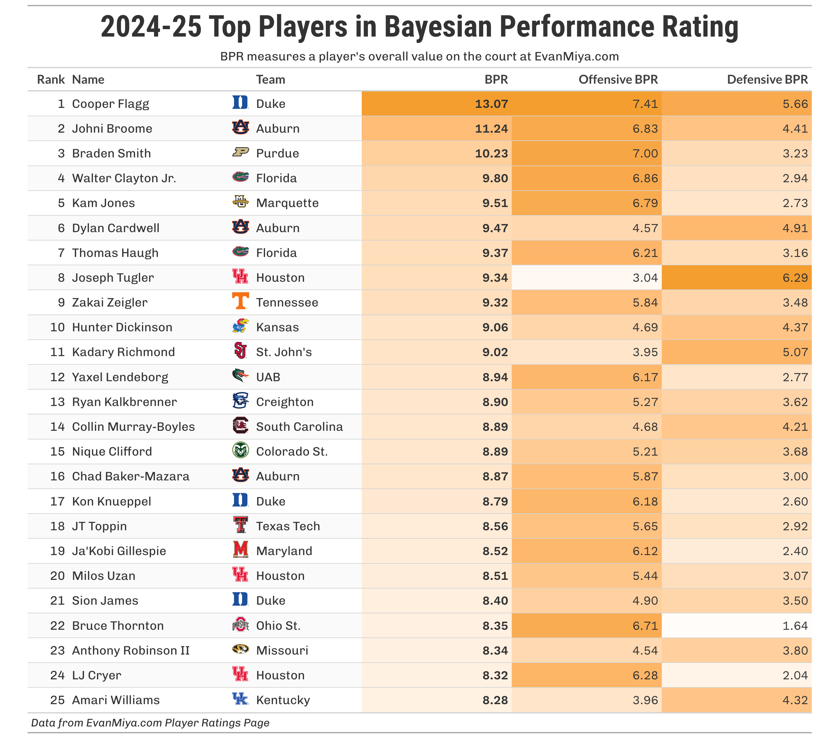
Enough technical details, let’s look at some numbers! The table below shows the top 25 players in BPR at the end of the 2024-25 season. In the top four, Flagg and Broome were clearly the best two players all season, and Braden Smith and Walter Clayton were consensus first-team All-Americans.
You can find the ratings for every other season on the Player Ratings page at EvanMiya.com, but I did want to take a look at the top 30 players all-time in BPR, going all the way back to 2009-10:
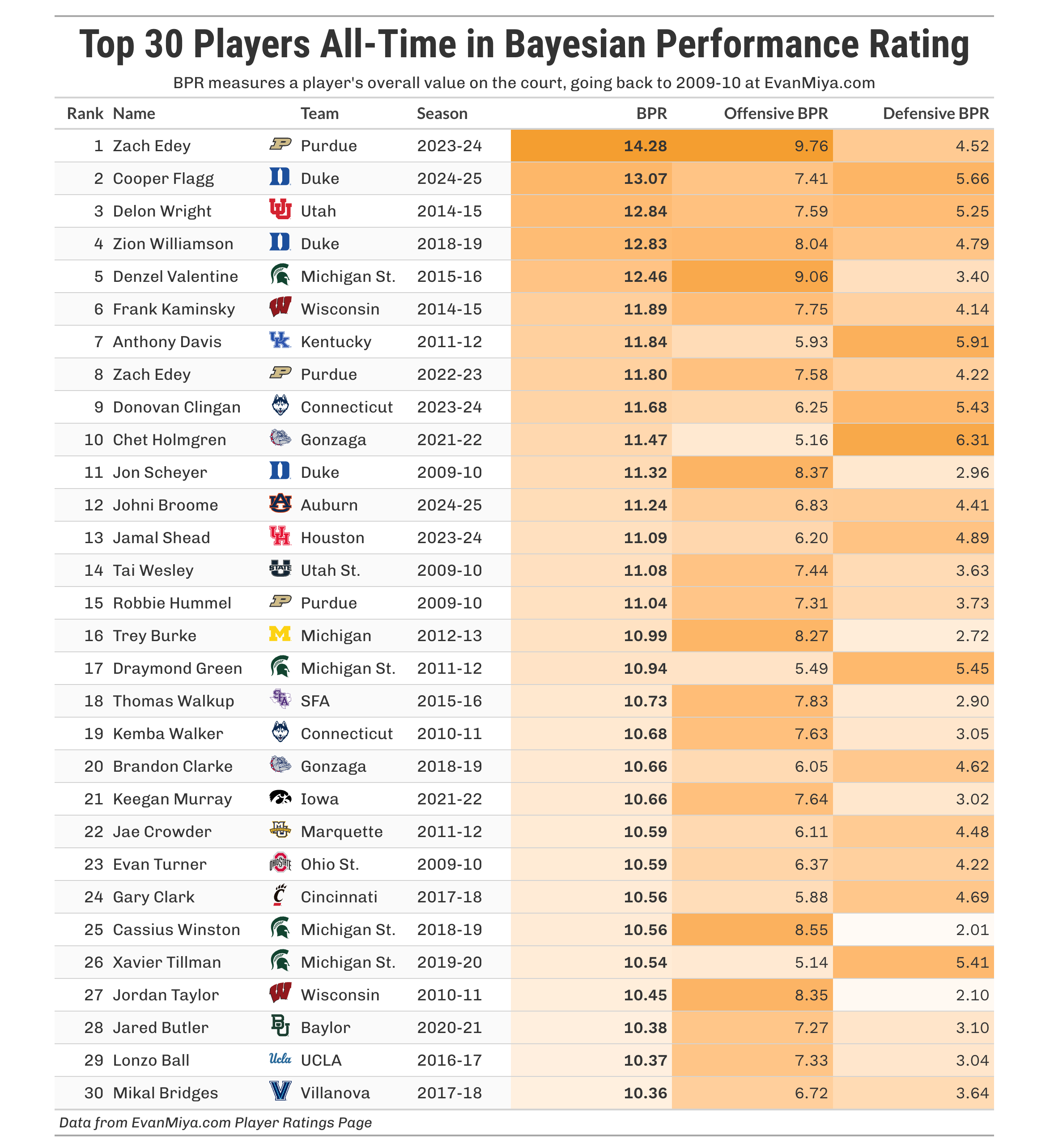
Zach Edey’s historic season in 2024 tops the list, followed by what Cooper Flagg just did last year in perhaps the most dominant season for a freshman ever. Zion Williamson’s lone season also makes the top five. Michigan State has four players in the top 30 all-time, the most of any team.
2025 Model Updates
For those who reference BPR regularly, I wanted to provide a brief list of the significant model updates for this upcoming season, although some have already been mentioned.
All data now goes back to the 2009-10 season, which you can find on the Player Ratings page.
I switched to using a 4-year RAPM college dataset, using several 4-year stints, to establish more accurate model tuning parameters. This led to updated shrinkage parameters, Box BPR stat weights, and overall weight given to box statistics vs on-court play-by-play data. The new model leans a little more heavily on the box score statistics, and the magnitude of the BPR values in a given year is also slightly higher than before.
The model more properly accounts for player minutes and usage and is not as biased against players who carry a big load like before. In the previous iteration, players who were on the court for a significant portion of their team’s possessions sometimes struggled to get the credit they deserved. For example, high usage guards like Devin Carter (2023-24), Walter Clayton (2024-25), and Bennett Stirtz (2024-25) have received significant boosts in the new model version.
Excellent players outside the high major ranks have also received significant bumps in some cases, such as Yaxel Lendeborg, DaRon Holmes II, and Jonathan Mogbo.
The preseason player projections model now includes two separate models based on whether a player is transferring or returning to his old team. Often, the variables that predict player success vary based on whether a player is returning to the same team and system or not. For example, advanced On-Off metrics are pretty useful for assessing player performance, but they are significantly less reliable for transfers.
Due to these updates, all previous season pages have been refreshed to reflect the new end-of-season BPR and Box BPR values using the latest model.
https://www.basketball-reference.com/about/per.html
https://www.basketball-reference.com/about/ratings.html
https://basketballstat.home.blog/2019/08/14/regularized-adjusted-plus-minus-rapm/
https://www.basketball-reference.com/about/bpm2.html
Learning a bit of bayesian modeling in school, and I was initially a bit confused on the reasoning for applying priors & bayesian thinking to player ratings but after reading it makes a lot of sense. This is brilliant.
Zach Edey appears in the all time list TWICE. I guess a lot of the top guys go straight to the NBA, but not a single one of the other guys turned in two Top 30 BPR performances?
So is it best all-time SEASONS/PEFORMANCES, then, and not best PLAYERS? Zach Edey is only one player.
I'm pretty sure.